Gene Expression Prediction
Published:
Pre-WGCNA
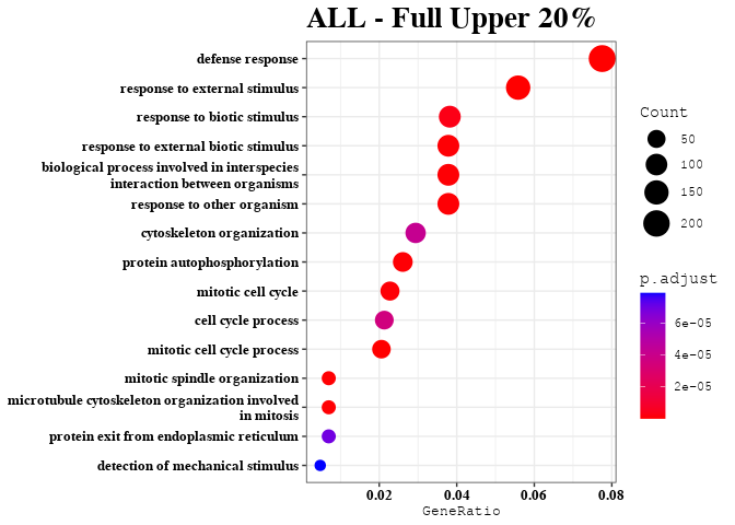
Treatment Effects on Gene Expression in Upper 20% of Predictable Gene Transcripts
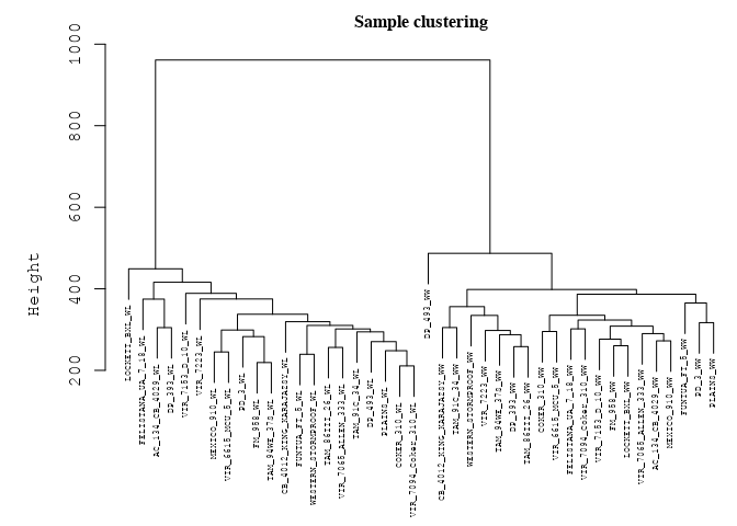
# Cluster tress (check if any outliers existed among
# samples)
datExpr_tree <- hclust(dist(datExpr), method = "average")
par(mar = c(0, 5, 2, 0))
plot(datExpr_tree, main = "Sample clustering", sub = "", xlab = "",
    cex.lab = 2, cex.axis = 1, cex.main = 1, cex.lab = 1, cex = 0.5)
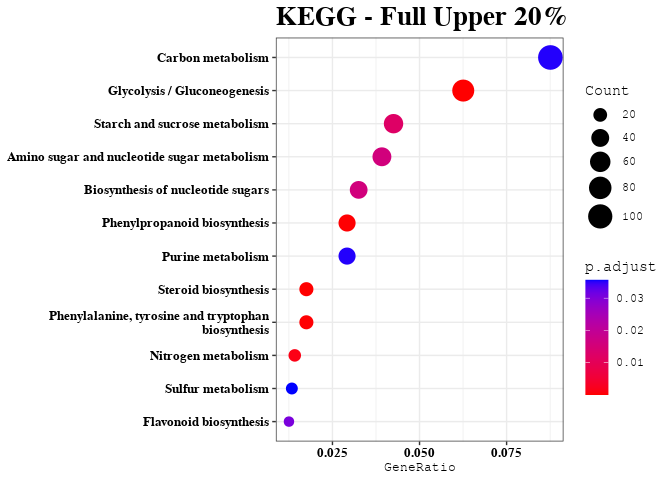
KEGG Analysis of Upper 20% of Predictable Gene Transcripts
length(dat)
enrichment_analysis(df = dat, plot_name = "Full Upper 20%")
WGCNA
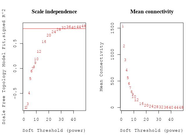
Soft thresholding
# Set powers to sample
powers = c(c(1:10), seq(from = 12, to = 50, by = 4))

# Call the network topology analysis function
sft = pickSoftThreshold(datExpr, powerVector = powers, verbose = 0)
k <- softConnectivity(datE = datExpr, power = sft$powerEstimate)
# Plot the results:
par(mfrow = c(1, 2))
cex1 = 0.9

# Scale-free topology fit index as a function of the
# soft-thresholding power
plot(sft$fitIndices[, 1], -sign(sft$fitIndices[, 3]) * sft$fitIndices[,
    2], xlab = "Soft Threshold (power)", ylab = "Scale Free Topology Model Fit,signed R^2",
    type = "n", main = paste("Scale independence"))
text(sft$fitIndices[, 1], -sign(sft$fitIndices[, 3]) * sft$fitIndices[,
    2], labels = powers, cex = cex1, col = "red")

# this line corresponds to using an R^2 cut-off of h
abline(h = 0.8, col = "red")

# Mean connectivity as a function of the soft-thresholding
# power
fig <- plot(sft$fitIndices[, 1], sft$fitIndices[, 5], xlab = "Soft Threshold (power)",
    ylab = "Mean Connectivity", type = "n", main = paste("Mean connectivity"))

text(sft$fitIndices[, 1], sft$fitIndices[, 5], labels = powers,
    cex = cex1, col = "red")
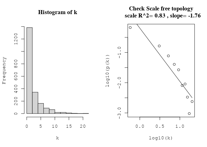
par(mfrow = c(1, 2))
hist(k)
scaleFreePlot(k, main = "Check Scale free topology\n")
Block-wise Network Construction & Module Detection
net = blockwiseModules(datExpr,
power = 30,
deepSplit=2,
TOMType = "unsigned",
reassignThreshold = 0,
maxBlockSize=440000,
# mergeCutHeight=0.10,
mergeCutHeight = 0.05,
numericLabels = TRUE,
pamRespectsDendro = FALSE,
verbose = 0,
pamStage=TRUE)
# corType="bicor")
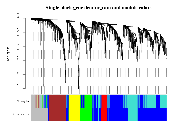
#Plot the dendogram with color assignment
moduleLabels = net$colors
moduleColors = labels2colors(net$colors)
MEs = net$MEs;
geneTree = net$dendrograms[[1]];
bwnet = blockwiseModules(datExpr,
power = 30,
deepSplit=2,
TOMType = "unsigned",
reassignThreshold = 0,
maxBlockSize=440000,
# mergeCutHeight=0.10,
mergeCutHeight = 0.05,
numericLabels = TRUE,
pamRespectsDendro = TRUE,
verbose = 0,
pamStage=TRUE)
# TOMDenom="mean",
# corType="bicor")
#Relabel blockwise modules
bwLabels = matchLabels(bwnet$colors, moduleLabels);
#Labels to colors for plotting
bwModuleColors = labels2colors(bwLabels)
#Compare the single block to the block-wise network analysis
plotDendroAndColors(geneTree,cbind(moduleColors, bwModuleColors), c("Single", "2 blocks"), main = "Single block gene dendrogram and module colors", dendroLabels = FALSE, hang = 0.03, addGuide = TRUE,guideHang = 0.05)
singleBlockMEs = moduleEigengenes(datExpr, moduleColors)$eigengenes
blockwiseMEs = moduleEigengenes(datExpr, bwModuleColors)$eigengenes

single2blockwise = match(names(singleBlockMEs), names(blockwiseMEs))
signif(diag(cor(blockwiseMEs[, single2blockwise], singleBlockMEs)),
    3)
##      MEblue     MEbrown     MEgreen      MEgrey       MEred MEturquoise
##       0.991       1.000       0.998       0.993       1.000       0.987
##    MEyellow
##       1.000
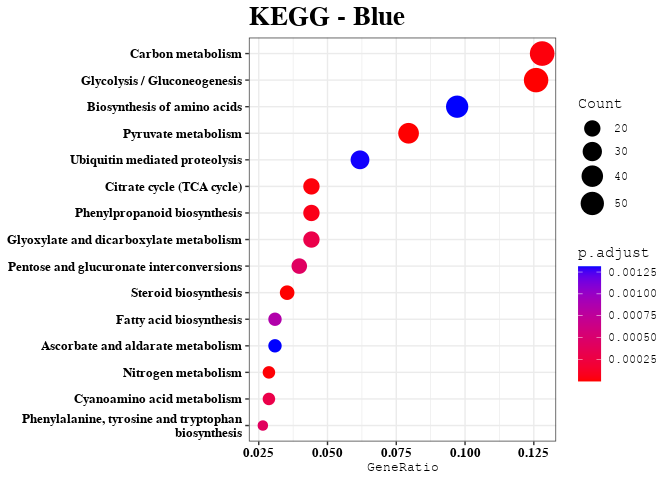
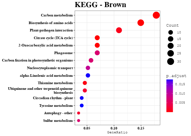
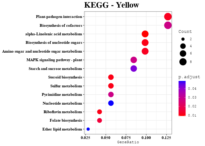
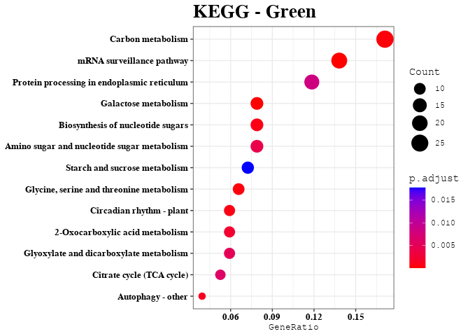
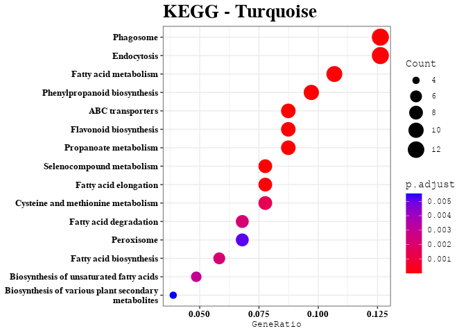
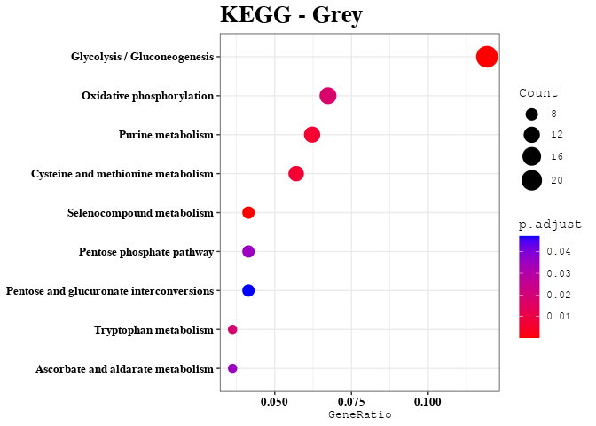
Enrichment Analyses
out <- data.frame(gene = colnames(datExpr), module = bwModuleColors)

mods = unique(bwModuleColors)
go_list = c()
kegg_list = c()
mkegg_list = c()


for (mod in mods) {
    temp = subset(out, module == mod)
    result = filter(dat, dat$Gene %in% temp$gene)
    result = enrichment_analysis(df = result, plot_name = mod)

    try({
        # print(result$go_plot)
        print(result$kegg_plot)
        # print(result$mkegg_plot)

        go_res = result$go_data
        go_list[[mod]] = go_res@result$Description

        kk_res = result$kegg_data
        kegg_list[[mod]] = kk_res@result$Description

        # mkk_res = result$mkegg_data mkegg_list[[mod]] =
        # mkk_res@result$Description

    }, silent = TRUE)

}